MCS 275 Spring 2023 Worksheet 10 Solutions
- Course instructor: Emily Dumas
- Contributors to this document: Emily Dumas, Kylash Viswanathan
Topics
This worksheet is about numpy.
Resources
These things might be helpful while working on the problems. Remember that for worksheets, we don't strictly limit what resources you can consult, so these are only suggestions.
- VanderPlas:
- Chapter 2 covers numpy
- Course sample code repo
- Lecture 22 - numpy
- Lecture 23 - numpy 2
- Lecture 24 - Julia sets
- Downey's book
Notebook recommended
I think you'll have the best experience with this worksheet if you do your work in a Python notebook.
Also, remember to install numpy (and pillow, if you haven't already). For most people thse commands will do it:
python3 -m pip install numpy
python3 -m pip install pillow
1. Generate these arrays
Try to find concise expressions that generate these numpy arrays, without using explicit loops and without listing all the elements out as literals.
A.
array([ 4, 9, 16, 25, 36, 49, 64, 81, 100, 121])B.
array([ 0.2, 0.4, 0.6, -5. , -5. , -5. , -5. , -5. , 1.8, 2. , 2.2, 2.4, 2.6, 2.8, 3. , 3.2, 3.4, 3.6])C.
array([[4., 3., 2., 1., 0., 1., 2., 3., 4.],
       [4., 3., 2., 1., 0., 1., 2., 3., 4.],
       [4., 3., 2., 1., 0., 1., 2., 3., 4.],
       [4., 3., 2., 1., 0., 1., 2., 3., 4.],
       [4., 3., 2., 1., 0., 1., 2., 3., 4.],
       [4., 3., 2., 1., 0., 1., 2., 3., 4.],
       [4., 3., 2., 1., 0., 1., 2., 3., 4.]])
D.
array([[7, 0, 7, 7, 7, 7, 7, 7, 0, 7],
       [0, 0, 0, 0, 0, 0, 0, 0, 0, 0],
       [7, 0, 7, 7, 7, 7, 7, 7, 0, 7],
       [7, 0, 7, 7, 7, 7, 7, 7, 0, 7],
       [7, 0, 7, 7, 7, 7, 7, 7, 0, 7],
       [7, 0, 7, 7, 7, 7, 7, 7, 0, 7],
       [0, 0, 0, 0, 0, 0, 0, 0, 0, 0],
       [7, 0, 7, 7, 7, 7, 7, 7, 0, 7]])
Solutions
A.
import numpy as np

A = np.arange(2,12)**2
A
B.
B = np.arange(0.2,3.8,0.2)
B[3:8] = -5
B
C.
C = np.abs(np.zeros((7,9)) + np.arange(-4,5))
C
D.
D = np.full((8,10),7,dtype="int64")
D[1]=0
D[-2]=0
D[:,1]=0
D[:,-2]=0
D
2. Numpy image processing
Here is a grayscale photograph of an onion sitting on a wooden desk.
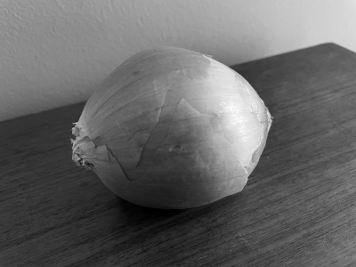
In this problem, you'll work with the data from this image using numpy. Last week, you did some image processing using .getpixel and .putpixel from Pillow, but converting the image to a numpy array and then analyzing the data using numpy is really a better approach in most cases.
Here are two functions that will help with that: One loads a PNG image into a numpy array. It requires numpy and PIL. If the PNG image is grayscale, you'll get a 2-dimensional array whose dtype is uint8. The other saves a 2-dimension numpy array with dtype uint8 as a PNG image.
import PIL.Image
import numpy as np

def load_image_to_array(fn):
    "Open image file with name `fn` and return as a numpy array`"
    img = PIL.Image.open(fn)
    return np.array(img)

def save_array_to_image(fn,A):
    "Save 2D array `A` with dtype `uint8` to file named `fn`"
    assert A.ndim == 2
    assert A.dtype == np.dtype("uint8")
    img = PIL.Image.fromarray(A)
    img.save(fn)
A. Peak onion
What row of the image has the largest average brightness?
What column has the largest average brightness?
What is the brightest color that appears in the image? Where does it appear?
Solution
# load the image, and obtain the dimensions.
from PIL import Image
onion = load_image_to_array("ws10_grayscale_onion.png")
Row with the largest average brightness:
row_means = np.mean(onion, axis = 1) # obtains the means of the rows
np.argmax(row_means)
Column with the largest average brightness
col_means = np.mean(onion, axis = 0) # obtains the means of the columns
np.argmax(col_means)
Brightest color that appears in the image and Location
# Obtain index of maximium value
# The index returned is an integer, giving the position
# of the maximum in the 1D array obtained by joining
# all the rows together, one after another
max_idx = np.argmax(onion)

# Obtain the corresponding row and column

# Each row has onion.shape[1] items, so the number of times
# this divides max_idx will be the row number.
max_row = max_idx // onion.shape[1]  # each row has onion.shape[1] items

# Each row has onion.shape[1] items, so the remainder when
# dividing max_idx by that will be the column number.
max_col = max_idx % onion.shape[1]

print("Indices of brightest color", max_row,max_col)
print("Brightest color", onion[max_row][max_col])

# Confirm that this is the true maximum
# Using .ravel() which reshapes an ND array to 1D
# (we didn't cover this function, and you don't need to know about it)
assert onion[max_row][max_col] == onion.ravel()[max_idx]
B. Horizontal average
Create a new grayscale image file ws10_grayscale_onion_colavg.png with the same dimensions as the original image, but where each column is filled with a solid color that is as close as possible to the average brightness of the coresponding column of the original image. The result should look like this:

Hint: If you have an array of floats you can convert them to an array of uint8 values using the method call .astype("uint8").
Apology from Prof. Dumas
Given what they were asking, I should have called part B "vertical average" and part C "horizontal average". The pictures match what the questions ask you to do, but the titles were switched. Sorry about that.
Solution
onion_colavg = (np.zeros_like(onion) + np.mean(onion,axis=0)).astype("uint8")
save_array_to_image("ws10_grayscale_onion_colavg.png",onion_colavg)
C. Vertical average
Create a new grayscale image file ws10_grayscale_onion_rowavg.png with the same dimensions as the original image, but where each row is filled with a solid color that is as close as possible to the average brightness of the coresponding row of the original image. The result should look like this:

Solution
onion_rowavg = (np.zeros_like(onion) + np.mean(onion,axis=1).reshape((300,1))).astype("uint8")
save_array_to_image("ws10_grayscale_onion_rowavg.png",onion_rowavg)
D. Gamma adjust
If you divide a grayscale image array by $255.0$, you get an array of floats between $0.0$ and $1.0$. If you raise those floats to a power $\gamma$ (usually chosen to be near $1$) and then multiply by $255.0$ again, the resulting image will be "gamma adjusted" by exponent $\gamma$. Of course if $\gamma=1$ you just get the original image back again.
Apply this process to the onion photo with for each of these values of $\gamma$:
- 0.25
- 0.7
- 1.0
- 1.2
- 1.4
- 2
- 5
How would you explain the qualitative effect of changing $\gamma$?
Solution
The images are shown below. The effect of $\gamma$ is to darken or lighten the image, but in a way that still makes full black or full white remain possible. Lower values of $\gamma$ give brighter images.
gamma = 0.25
PIL.Image.fromarray((((onion/255.0)**gamma)*255.0).astype("uint8"))

gamma = 0.7
PIL.Image.fromarray((((onion/255.0)**gamma)*255.0).astype("uint8"))

gamma = 1 # same as original image, in fact
PIL.Image.fromarray((((onion/255.0)**gamma)*255.0).astype("uint8"))

gamma = 1.2
PIL.Image.fromarray((((onion/255.0)**gamma)*255.0).astype("uint8"))

gamma = 1.4
PIL.Image.fromarray((((onion/255.0)**gamma)*255.0).astype("uint8"))

gamma = 2
PIL.Image.fromarray((((onion/255.0)**gamma)*255.0).astype("uint8"))

gamma = 5
PIL.Image.fromarray((((onion/255.0)**gamma)*255.0).astype("uint8"))

3. Riemann Sum
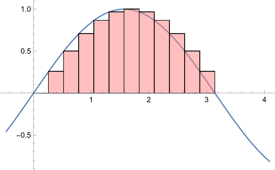
The area under one "hump" of the sine function is exactly 2, i.e. $$ \int_0^\pi \sin(x) \, dx = 2 $$
For any positive integer n, that integral can be approximated by dividing the interval $[0,\pi]$ into n equal parts and forming a left-endpoint Riemann sum, whereby the area is approximated by a union of n rectangles. This is shown below for n=12:
Here's a function that computes the Riemann sum naively, using Python for loops:
import math
import time
def naive_rs(n):
    """
    Riemann sum for sin(x) on [0,pi] computed without numpy
    and without any concern for accumulating errors when you
    sum many small floats. (TODO: Learn numerical analysis!)
    """
    hsum = 0.0
    for i in range(n):
        hsum += math.sin(math.pi*(i/n)) # Add a rectangle height
    return hsum * (math.pi/n) # Multiply sum of heights by width
As we can see, the return value gets quite close to 2 as we increase n.
naive_rs(3)
naive_rs(5)
naive_rs(5_000_000)
However, for large values of n this function is quite slow. (Try n=5_000_000 or n=20_000_000 for example.)
Write a function numpy_rs(n) that makes an equivalent computation using numpy to avoid explicit iteration.
Check that numpy_rs(n) and naive_rs(n) return values that are extremely close for small values of n. (They can't be expected to necessarily agree exactly, as floating point addition is not associative.)
Then compare the speed of numpy_rs(n) and naive_rs(n) for large values of n. (For this problem, let's say a value of n is "large" if the slower of the two calculations takes at least half a second.)
Hints: You won't need the math module at all in the numpy solution. There's a constant called np.pi that is equal to $\pi$. The solution won't contain any loops.
Solution
def numpy_rs(n):
    "Riemann sum for sin(x) on [0,pi] with numpy"
    return np.sum(np.sin(np.pi*np.linspace(0,1,n+1)))*np.pi/n
# Implementation of numpy's integration via Riemann Sums
t0 = time.time()
numpy_rs(5_000_000)
print(time.time()-t0)
# Implementation of naive integration via Riemann Sums
t0 = time.time()
naive_rs(5_000_000)
print(time.time()-t0)
For a moderately sized integration, the numpy version performs nearly 7 times faster
Extra challenge
If you have extra time: Generalize numpy_rs(n) to a function numpy_rs(f,a,b,n) which takes a function f, interval endpoints a and b, and a number of rectangles n, and computes the Riemann sum approximation of $\int_a^b f(x) \,dx$ using numpy. Assume f is a numpy ufunc, so it can be applied directly to an array.
Revision history
- 2023-03-14 - Initial publication