Lecture 18
Comparison sorts
MCS 275 Spring 2022
Emily Dumas
Lecture 18: Comparison sorts
Course bulletins:
- Homework 6 due at Noon tomorrow.
- Project 2 due 6pm Friday. Autograder open.
- I cannot promise any availability between 1pm and 6pm on Friday. Plan accordingly.
- Worksheet 7 coming soon.
- Starting new topic (trees) on Wednesday.
Growth rates
Let's look at the functions $n$, $n \log(n)$, and $n^2$ as $n$ grows.
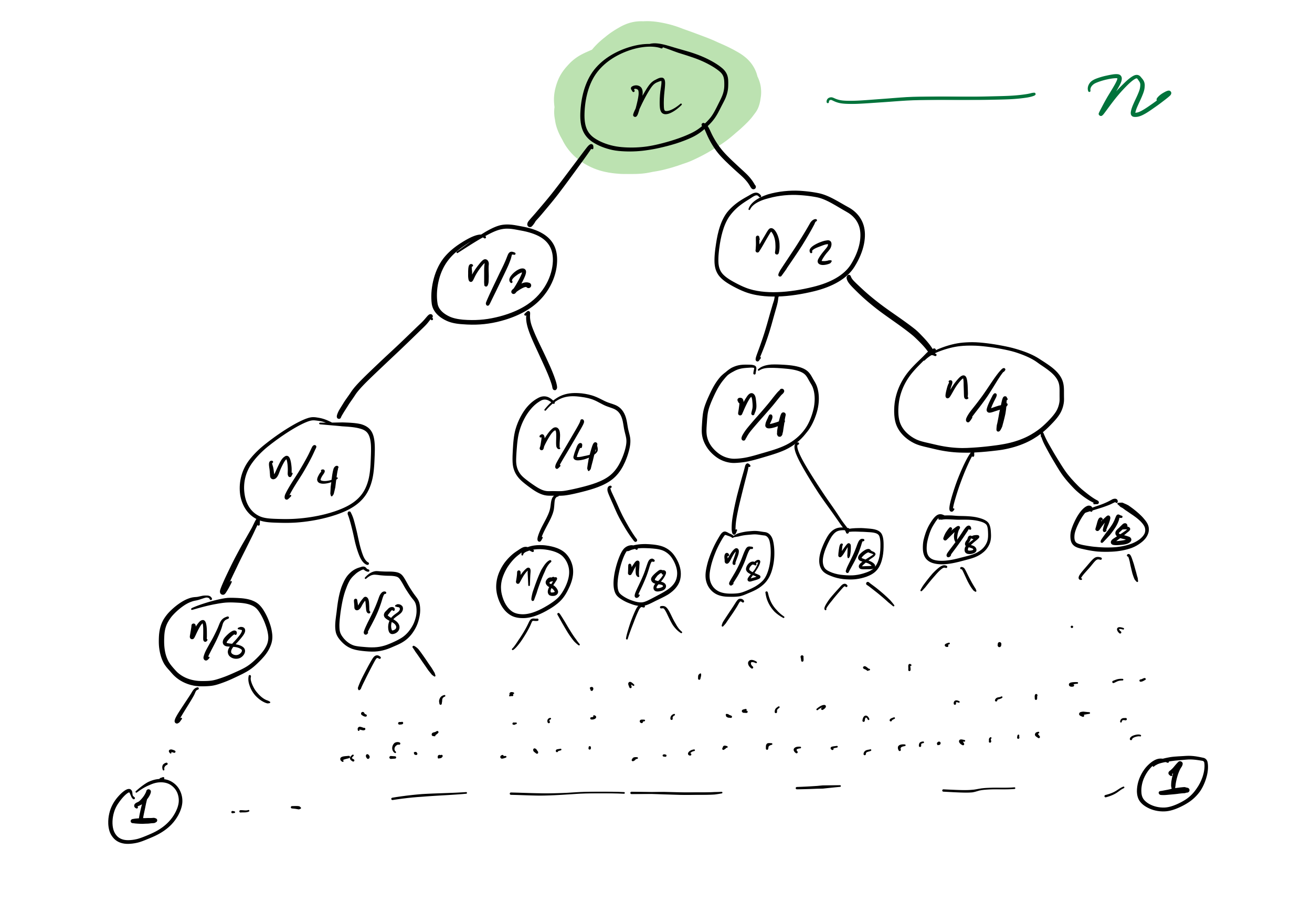
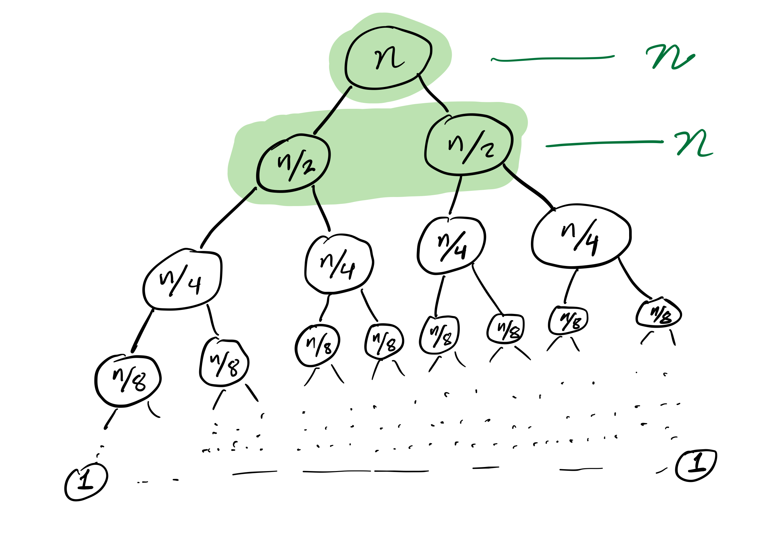
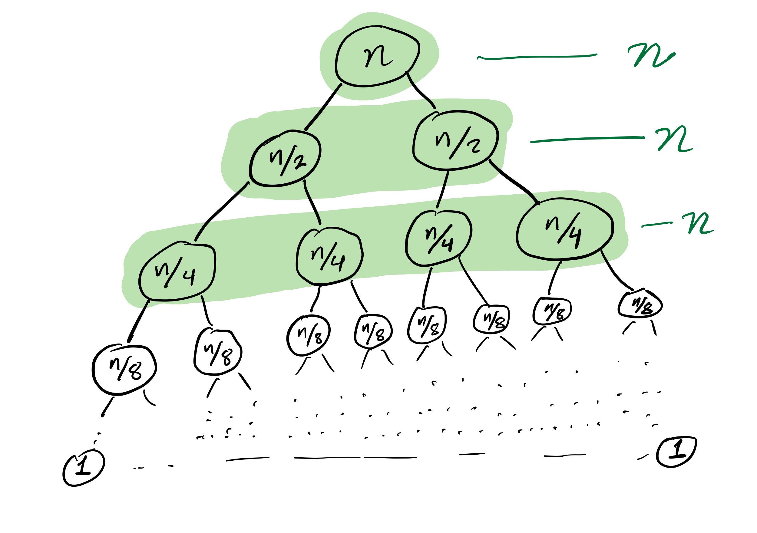
Mergesort recursion tree
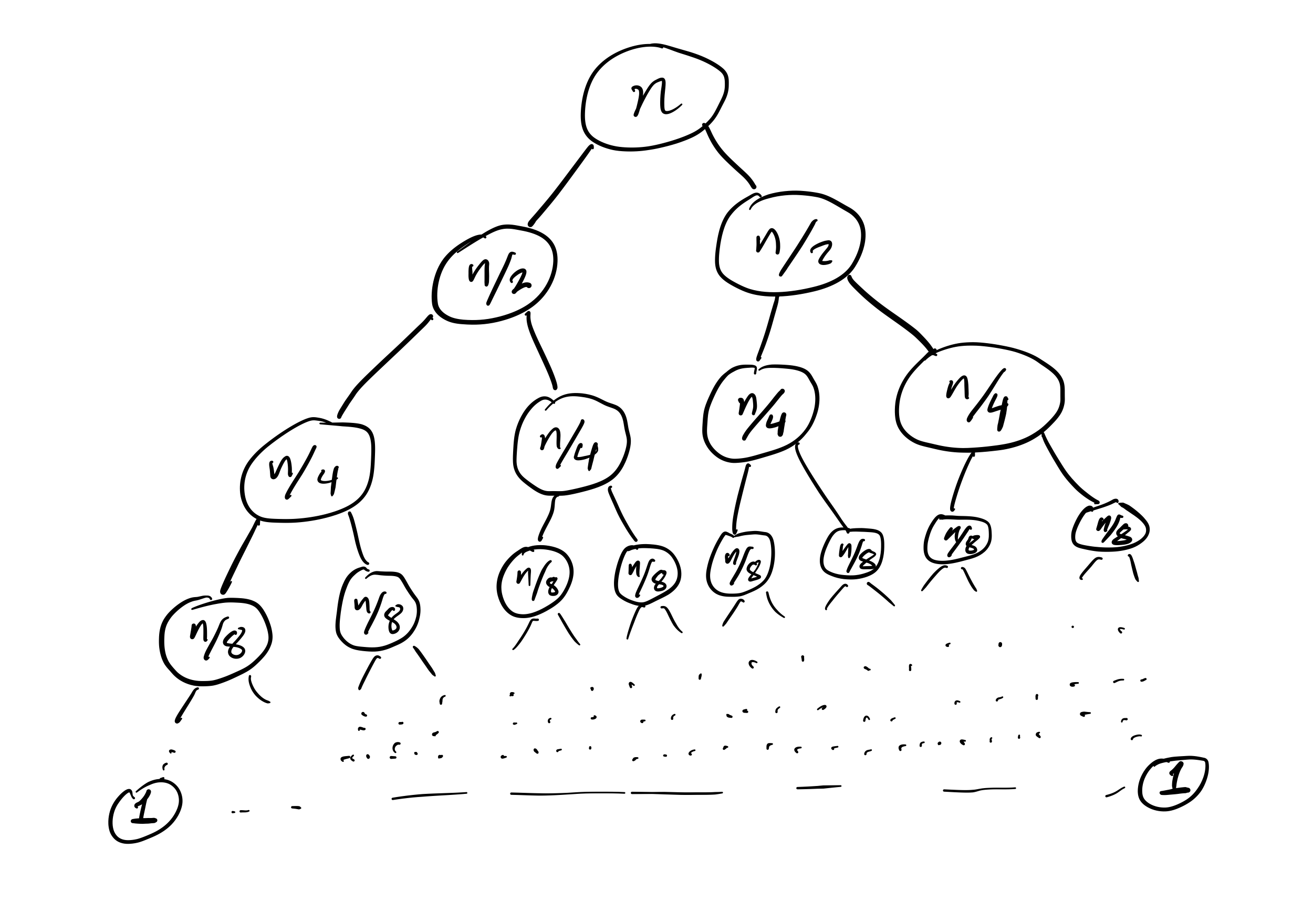
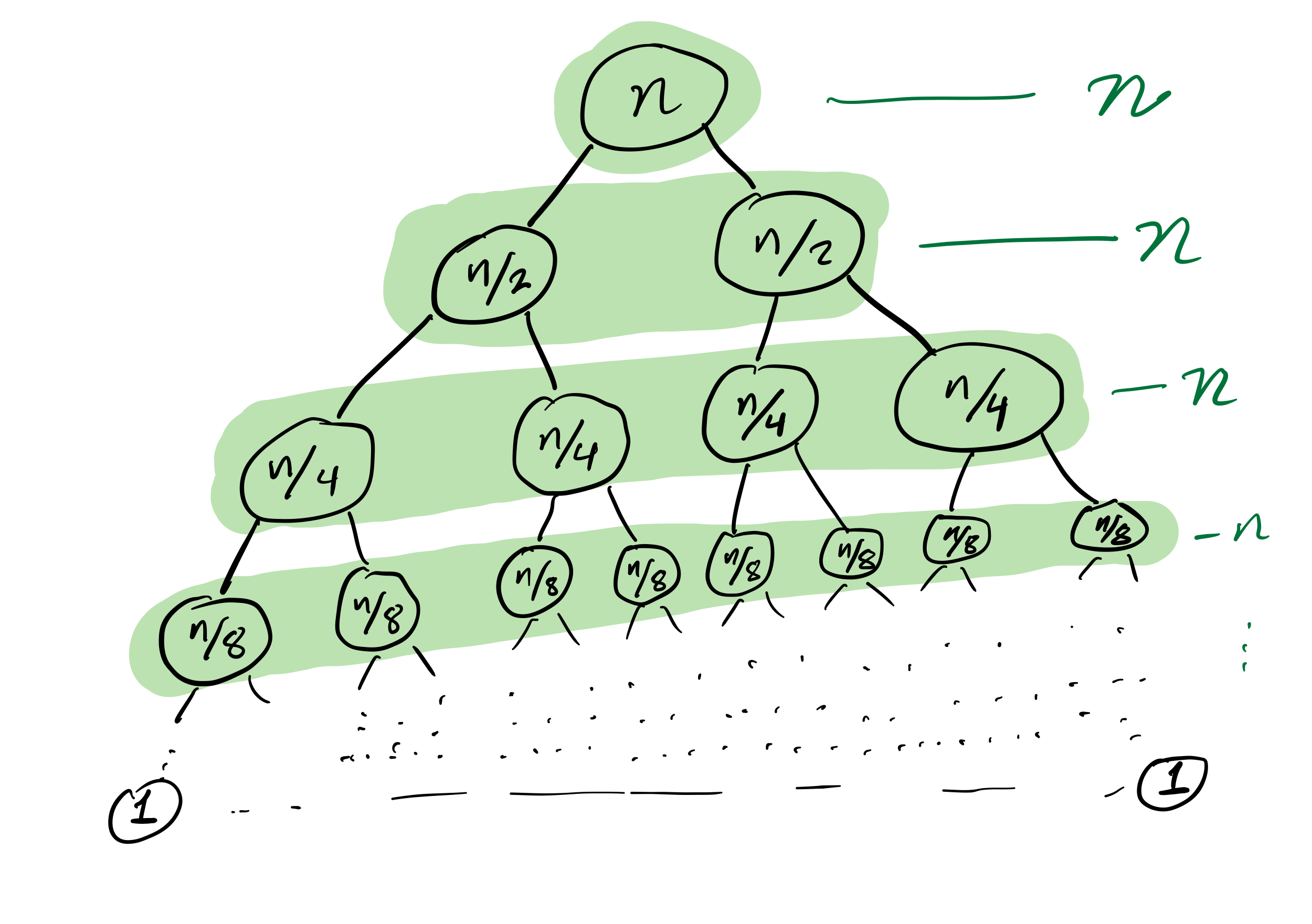
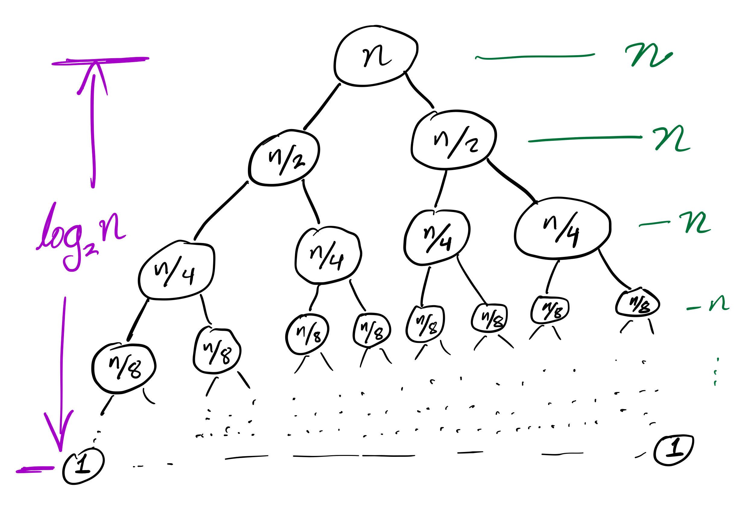
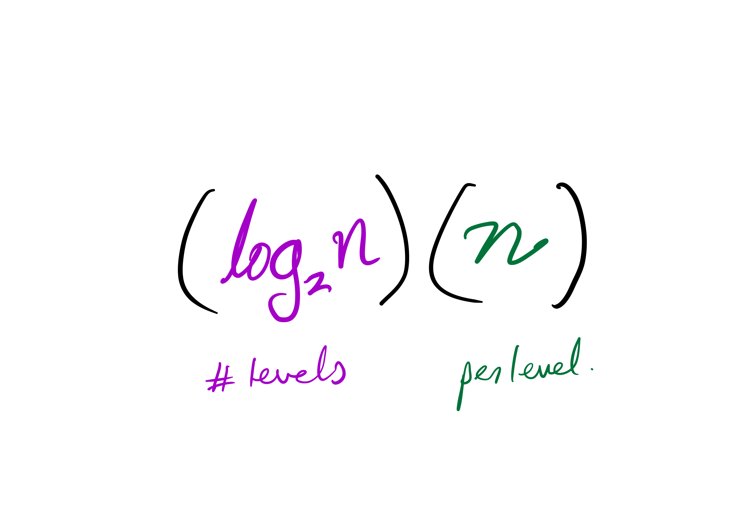
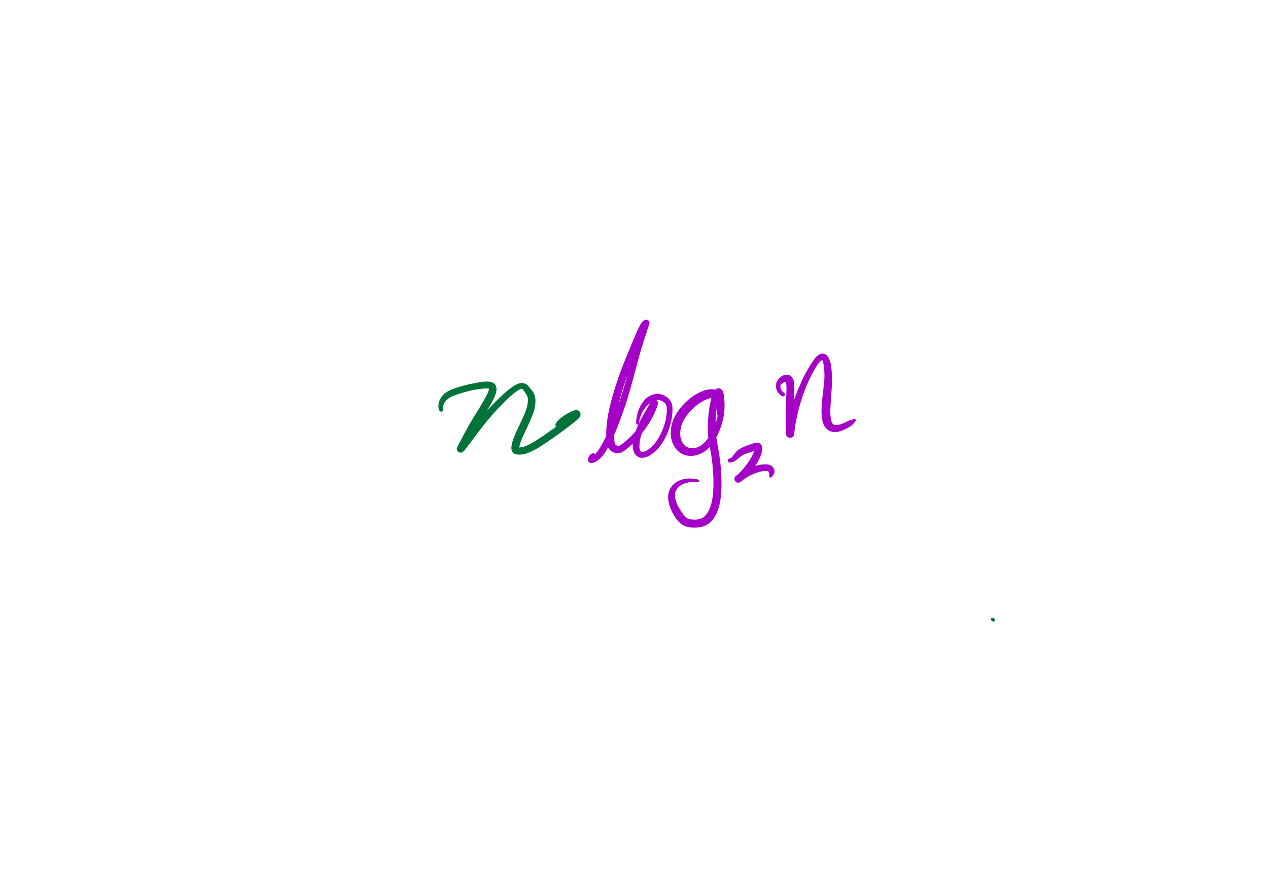
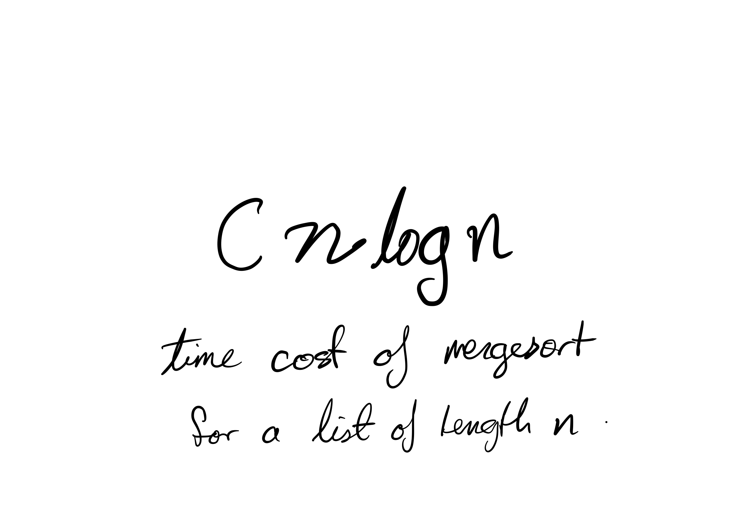
Efficiency
Theorem: If you measure the time cost of mergesort in any of these terms
- Number of comparisons made
- Number of assignments (e.g.
L[i] = xcounts as 1) - Number of Python statements executed
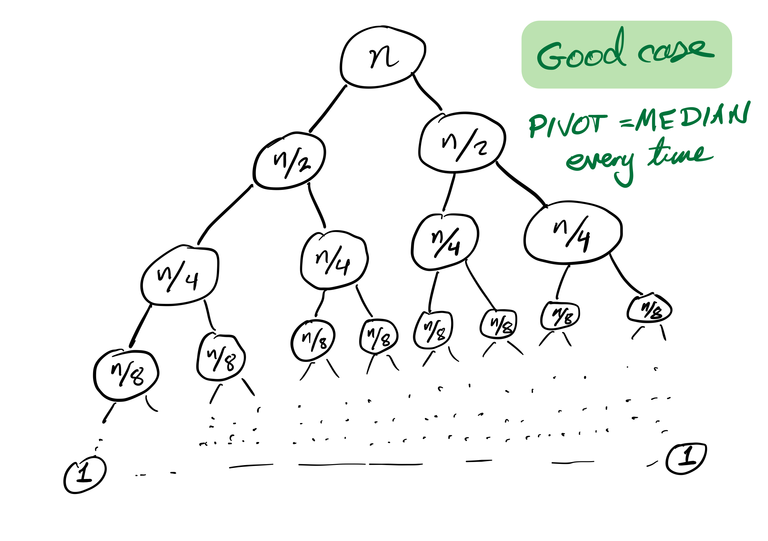
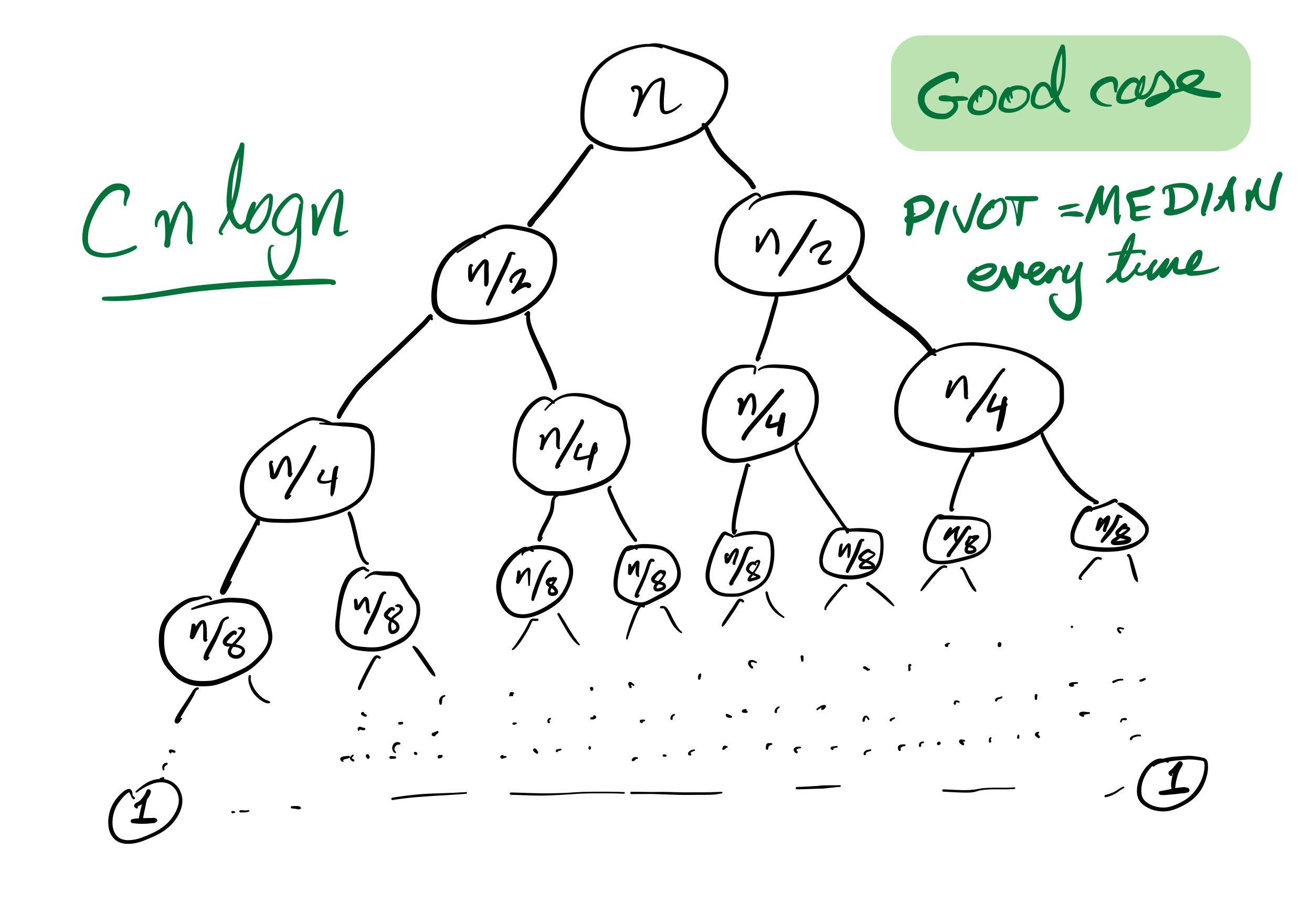
then the cost to sort a list of length $n$ is less than $C n \log(n)$, for some constant $C$ that only depends on which expense measure you chose.
Looking back on quicksort
It ought to be called partitionsort because the algorithm is simply:
- Partition the list
- Quicksort the part before the pivot
- Quicksort the part after the pivot
Other partition strategories
We used the last element of the list as a pivot. Other popular choices:
- The first element,
L[start] - A random element of
L[start:end] - The element
L[(start+end)//2] - An element near the median of
L[start:end](more complicated to find!)
How to choose?
Knowing something about your starting data may guide choice of partition strategy (or even the choice to use something other than quicksort).
Almost-sorted data is a common special case where first or last pivots are bad.
Efficiency
Theorem: If you measure the time cost of quicksort in any of these terms
- Number of comparisons made
- Number of swaps or assignments
- Number of Python statements executed
then the cost to sort a list of length $n$ is less than $C n^2$, for some constant $C$.
But if you average over all possible orders of the input data, the result is less than $C n \log(n)$.
Quicksort recursion tree
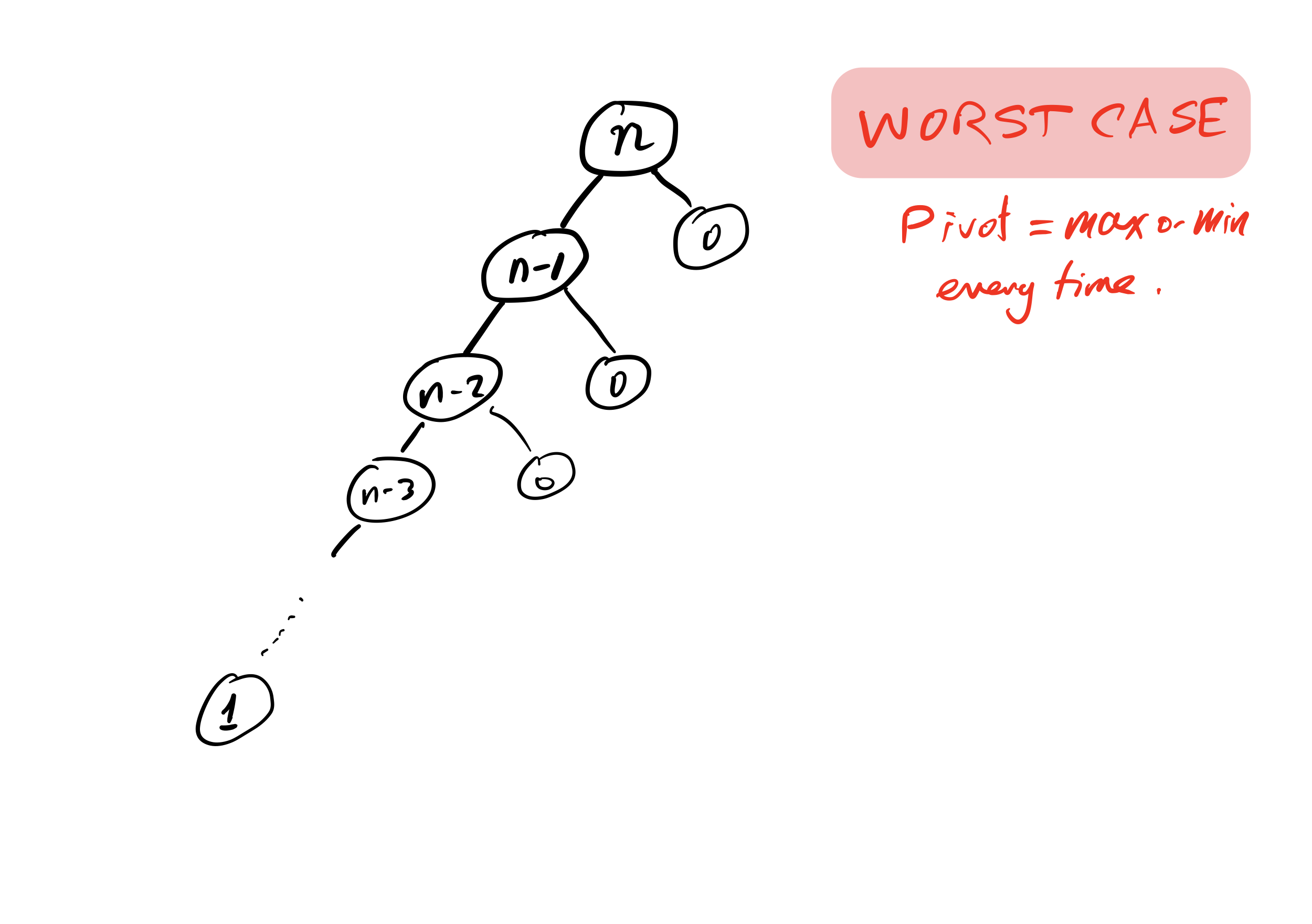
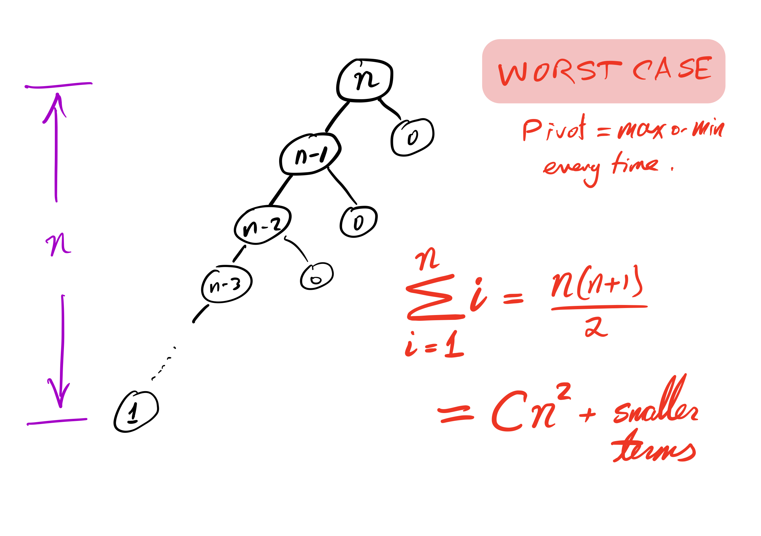
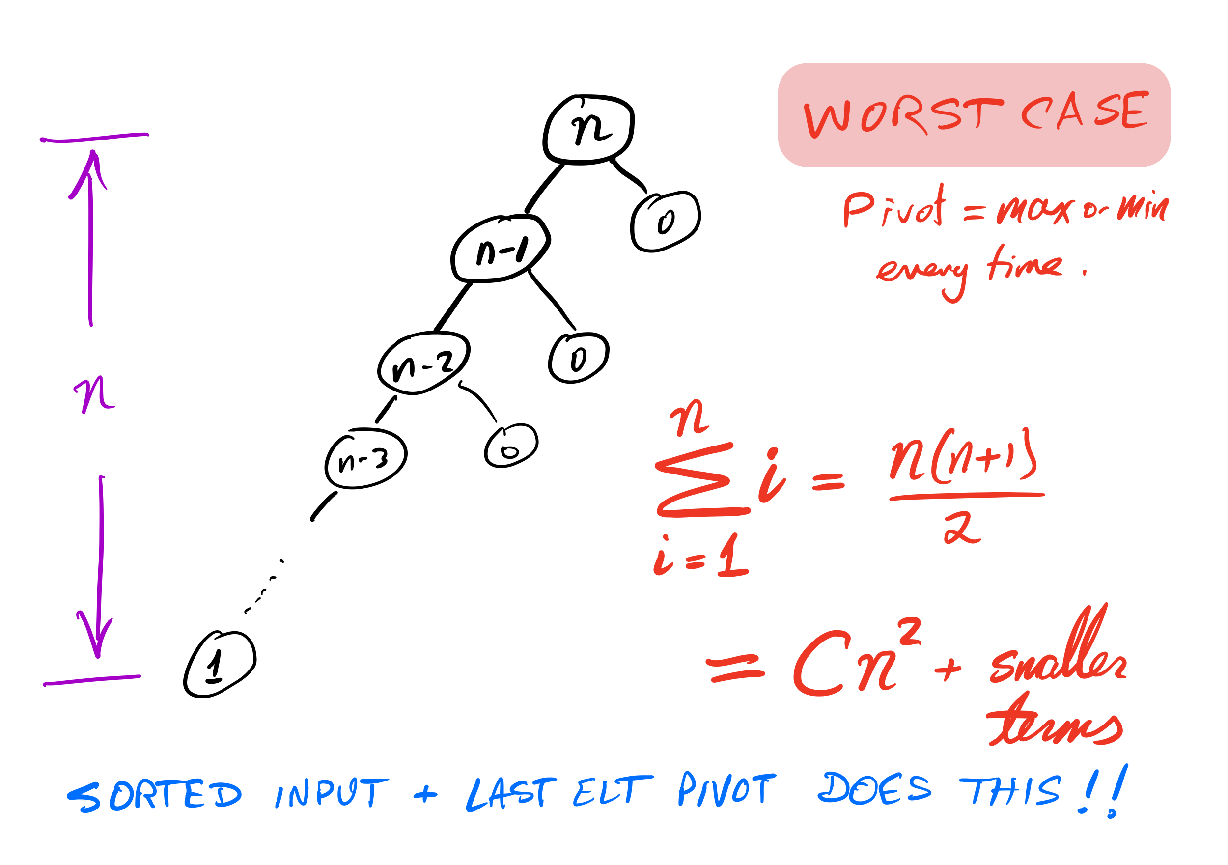
Bad case
What if we ask our version of quicksort to sort a list that is already sorted?
Recursion depth is $n$ (whereas if the pivot is always the median it would be $\approx \log_2 n$).
Number of comparisons $\approx C n^2$. Very slow!
Stability
A sort is called stable if items that compare as equal stay in the same relative order after sorting.
This could be important if the items are more complex objects we want to sort by one attribute (e.g. sort alphabetized employee records by hiring year).
As we implemented them:
- Mergesort is stable
- Quicksort is not stable
Efficiency summary
| Algorithm | Time (worst) | Time (average) | Stable? | Space |
|---|---|---|---|---|
| Mergesort | $C n \log(n)$ | $C n\log(n)$ | Yes | $C n$ |
| Quicksort | $C n^2$ | $C n\log(n)$ | No | $C$ |
(Every time $C$ is used, it represents a different constant.)
Other comparison sorts
- Insertion sort — Convert the beginning of the list to a sorted list, starting with one element and growing by one element at a time.
- Bubble sort — Process the list from left to right. Any time two adjacent elements are in the wrong order, switch them. Repeat $n$ times.
Efficiency summary
| Algorithm | Time (worst) | Time (average) | Stable? | Space |
|---|---|---|---|---|
| Mergesort | $C n \log(n)$ | $C n\log(n)$ | Yes | $C n$ |
| Quicksort | $C n^2$ | $C n\log(n)$ | No | $C$ |
| Insertion | $C n^2$ | $C n^2$ | Yes | $C$ |
| Bubble | $C n^2$ | $C n^2$ | Yes | $C$ |
(Every time $C$ is used, it represents a different constant.)
Closing thoughts on sorting
Mergesort is rarely a bad choice. It is stable and sorts in $C n \log(n)$ time. Nearly sorted input is not a pathological case. Its main weakness is its use of memory proportional to the input size.
Heapsort, which we may discuss later, has $C n \log(n)$ running time and uses constant space, but it is not stable.
There are stable comparison sorts with $C n \log(n)$ running time and constant space (best in every category!) though they tend to be more complex.
If swaps and comparisons have very different cost, it may be important to select an algorithm that minimizes one of them. Python's list.sort assumes that comparisons are expensive, and uses Timsort.
Quadratic danger
Algorithms that take time proportional to $n^2$ are a big source of real-world trouble. They are often fast enough in small-scale tests to not be noticed as a problem, yet are slow enough for large inputs to disable the fastest computers.
References
Unchanged from Lecture 17
- Making nice visualizations of sorting algorithms is a cottage industry in CS education. Some you might like to check out:
- 2D visualization through color sorting by Linus Lee
- Animated bar graph visualization of many sorting algorithms by Alex Macy
- Slanted line animated visualizations of mergesort and quicksort by Mike Bostock
Revision history
- 2022-02-21 Initial publication